Primary primitives

Boolean

Boolean primitives are a special type of primitive—they are created from other primitives (or shapes) that intersect with each other, as described in Boolean. Each member object of a Boolean primitive can only participate in one Boolean operation chain—the member objects cannot form interconnected networks.

BOOLEAN(member1, member2, operation, _Max_Angle_Threshold, _Angular_Deflection, _Linear_Deflection);

Member1 and member2 specify the member primitives (or shapes) of the Boolean operation.

Operation can be 0 (Cut), 1 (Union), or 2 (Intersection).

_Max_Angle_Threshold is a variable that specifies the maximum angle for the edges between the faces of the objects.

_Angular_Deflection is a variable that specifies the maximum angle between consecutive polyline segments.

_Linear_Deflection is a variable that specifies the maximum distance between a polyline and the face interior.

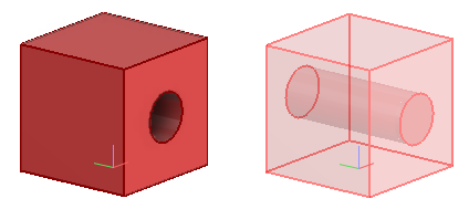
The example below shows the GDL source of a Boolean primitive whose members are a Box primitive and a Cylinder primitive.

Copy

Pnt17bzuW = POINT(-250,-250,0); 
Dir17bzuW = DIRECTION(1,0,0); 
Dir17bzuV = DIRECTION(0,1,0); 
Box17bzue = PIPED(Pnt17bzuW,Dir17bzuW,Dir17bzuV,500,500,500); 
Pnt17bzzi = POINT(0,-275,250); 
Pnt17c004 = POINT(0,275,250); 
Cyl17c005 = CYLINDER(Pnt17bzzi,Pnt17c004,100,0); 
_Max_Angle_Threshold = 40;
_Angular_Deflection = 1.5;
_Linear_Deflection = 4;
Boo17c00T = BOOLEAN(Box17bzue,Cyl17c005,0,_Max_Angle_Threshold,
_Angular_Deflection,_Linear_Deflection);

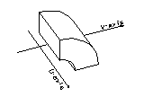
Box

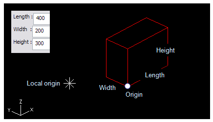
PIPED(p1, x_dir, y_dir, x_side, y_side, z_side);

Point p1 positions one corner of the box. From that corner x_side goes in the direction of x_dir and y_side in the direction of y_dir. An implicit z_dir is generated from x_dir y_dir, so that the resulting coordinate system is right-handed. Directions x_dir and y_dir must be orthogonal.

/* example of BOX */

x_axis = DIRECTION(1,0,0);

y_axis = DIRECTION(0,1,0);

length = 400;

width = 200;

height = 300;

p1 = POINT(320,-50,0);

exp_box = PIPED(p1,x_axis,y_axis,length,width,height);

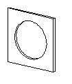
Plate

PLATE(p1, dir_thick, dir_x, sect, thickness);

PLATE(p1, dir_thick, rotation, sect, thickness)

In both cases p1 defines the origin of the section sect. The plate is oriented so that its thickness grows in the direction of dir_thick from point p1. The direction of the local x-axis of the section is either given or it is rotated rotation radians around the dir_thick axis from its default direction. The default direction for the local x-axis is such that it is parallel to the global XY-plane. In the default position the local y-axis points upwards.

/* This example shows use of primitive PLATE */

p1 = POINT(0,0,0);

x_axis = DIRECTION(1,0,0);

y_axis = DIRECTION(0,1,0);

c = atan(1)/45;

curve1 = CURVE(0,0,1000,0,1000,1000,0,1000);

curve2 = CURVE(250,250, arc,500,500,360*c);

sect = SECTION(curve1,curve2,0,0);

exp_plate = PLATE(p1,x_axis,y_axis,sect,50);

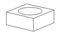
Sweep

SWEEP(p1,p2, x_dir, sect);

SWEEP(p1,p2, rotation, sect);

Sweep volumes describe the volume covered by moving a profile shape through space perpendicular to the profile plane. It can be considered to be a (usually) very thick plate. Points p1 and p2 define the endpoints of the sweep. The origin of the cross-section sweeps from p1 to p2. The ends will be orthogonal in the direction p1p2. Directions for the local x and y directions are defined in the same way as for plates.

/* This example shows use of primitive SWEEP */

p1 = POINT(0,0,0);

p2 = POINT(0,0,400);

x_axis = DIRECTION(1,0,0);

c = atan(1)/45;

curve1 = CURVE(0,0,1000,0,1000,1000,0,1000);

curve2 = CURVE(250,250, arc,500,500,360*c);

sect = SECTION(curve1,curve2,0,0);

exp_sweep = SWEEP(p1,p2,x_axis,sect);

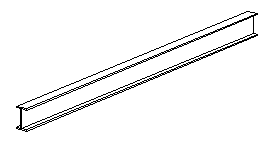
Beam

BEAM(p1, p2, x_dir, beam_number);

BEAM(p1,p2, rotation, beam_number);

The declaration for beam is parametric, since the declaration refers to the beam library, which contains cross-section shapes for beams. In other words the actual appearance of a beam depends on the beam library. Orientation of the beam is defined in the same way as sweeps.

/* example of using BEAM in gdl definition */

y_axis = DIRECTION(0,1,0);

p1 = POINT(0,0,0);

p2 = POINT(2000,0,0);

be_number = 202903;

exp_beam = BEAM(p1,p2,y_axis,be_number);

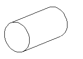
Cylinder

CYLINDER(p1, p2, r, t);

Points p1 and p2 are the endpoints of the cylinder. The radius is r and the wall thickness is t. The inside is not visualized.

/* This file shows how to create a CYLINDER */

length = 200;

diam = 100;

p1 = POINT(0,0,0);

p2 = POINT(length,0,0);

exp_cyli = CYLINDER(p1,p2,diam/2,1);

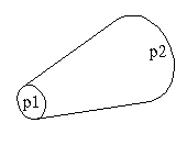
Cone

CONE(p1, p2, radius1, radius2, t);

Points p1 and p2 are the cone's endpoints. The radius varies linearly from radius1 to radius2 as the cone sweeps from p1 to p2. The wall thickness is t.

/* this is a short example of the primitive CONE */

length = 100;

diam1 = 20;

diam2 = 50;

x_axis = DIRECTION(1,0,0);

p1 = POINT(0,0,0);

p2 = POINT(p1,x_axis,length);

expl_cone = CONE(p1,p2,diam1/2,diam2/2,1);

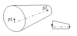
Eccentric Cone

EXCONE(p1, p2, dir, radius1, radius2, t);

Points p1 and p2 are the cone's endpoints. The direction dir points out from the starting plane defined by p1. The radius varies from radius1 to radius2 as the eccentric cone sweeps from p1 to p2. The wall thickness is t.

/* this is a short example of the primitive ECCENTRIC CONE */

diam1 = 50;

diam2 = 20;

x_neg = DIRECTION(-1,0,0);

p1 = POINT(0,0,0);

p2 = POINT(100,0,-15);

expl_excone = EXCONE(p1,p2,x_neg,diam1/2,diam2/2,1);

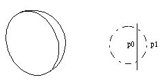
Sphere

SPHERE(p0, radius, t);

Point p0 defines the center of the sphere. The wall thickness is t.

/* This example introduces primitive SPHERE */

radius = 100;

walth = 0;

p1 = POINT(0,0,0);

exp_sph = SPHERE(p1,radius,walth);

Dish

DISH(p0, p1, r, t);

A dish is a spherical section obtained by one planar cut. The location of the dish is defined by two points p0 and p1. P0 gives the location of the center point of the cut plane. P1 defines the other (curved) end of the dish. The center point of the original sphere is located at distance r from point p1 in the direction p1p0. The wall thickness is t.

/* this example shows how to generate primitive geometry DISH */

radius = 1500;

walth = 1;

p0 = POINT(0,0,0);

p1 = POINT(1000,0,0);

exp_dish = DISH(p0,p1,radius,walth);

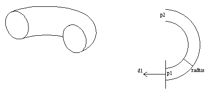
Toroid

TOROID(p1,p2, d, r, t);

An arc of a circle is defined by points p1 and p2 and vector d, which gives the direction of tangent at p1 that points out of the cut end of the arc. The toroid is generated by sweeping a (smaller) circle with the radius r along the arc from point p1 to point p2. The direction d then points out of the endplane defined by point p1. The wall thickness is t.

/* example of TOROID */

radius = 80;

walth = 1;

dir = DIRECTION(-1,0,0);

p1 = POINT(0,0,0);

p2 = POINT(0,400,0);

exp_toro = TOROID(p1,p2,dir,radius,walth);

Flange

FLANGE(p1, p2, diameter, d_hole);

Points p1 and p2 define the location and thickness of the flange. Point p1 defines the gasket surface. The hole is not drawn.

/* example of FLANGE */

diameter = 120;

d_hole = 100;

p1 = POINT(0,0,0);

p2 = POINT(20,0,0);

exp_fla = FLANGE(p1,p2,diameter,d_hole);

Surface of revolution

SURF_OF_REV(p0, u_ax, v_ax, r_curve, r_angle, close_vol, close_crv);

Creates a surface of revolution by rotating the given curve around a given line. Point p0 defines a point on the revolution axis. This point will also be the origin point of the u-v coordinate system of the curve. Direction u_ax defines the direction of the revolution axis and is also the u-axis of the curve coordinate system. Direction v_ax defines the direction of the v-axis of the curve coordinate system. r_curve identifies the curve that is used as the generating curve. r_angle is revolution angle. Positive direction is measured up from the u-v plane. If angle is 0 then creates a full revolution. close_vol can be set to 1 or 0. If 1 then creates a closed volume. Otherwise creates a shell. close_crv can also be 1 or 0. If set to 1 then the generating curve is used as a closed curve. If 0 then curve is used as open curve. There will be no connection line between the start point and end point of the curve.

/* example of SURF_OF_REV */

_UseDegrees = 1;

orig = POINT(0,0,0);

U_axis = DIRECTION(1,0,0);

V_axis = DIRECTION(0,1,0);

r_curve = CURVE(300,100, 300,250, 0,250, 0,100);

r_angle = 90;

close_vol = 1;

close_crv = 1;

srev = SURF_OF_REV(orig, U_axis, V_axis, r_curve, r_angle,

close_vol, close_crv);

3D model built by a Shape Script

SHAPE_BSV( "shape_name", orig, x_ax, y_ax [,param1, param2,...);

Creates a 3D model by calling a parameterized shape script. Point orig and directions x_ax and y_ax define the orientation of the local coordinate system of the shape model. There is a separate chapter that explains the details involved with shape scripts.

/* Example to create a shape */

_UseDegrees = 1;

p0 = POINT(0,0,0);

x_ax = DIRECTION(1,0,0);

y_ax = DIRECTION(0,1,0);

shape = SHAPE_BSV("CircleToRectangle", p0, x_ax, y_ax,

100, 300, 400, 500, 0, 0);

3D model built from inline BSV data

INLINE_BSV( orig, x_ax, y_ax, inline_data....);

Creates a 3D model by building a boundary surface volume (or surface) from inline data specified in numeric expressions that follow y_ax definition.

The following statements would create a polygon with a hole.

o = POINT(0,0,0);

x = DIRECTION(1,0,0);

y = DIRECTION(0,1,0);

bsv = INLINE_BSV(o, x, y,

8, 2, /* number of points and contours */

0, 0,0, /* points */

1000, 0, 0,

1000, 1000, 0,

0, 1000, 0,

200, 200, 0,

700, 200, 0,

700, 700, 0,

200, 700, 0,

4, 1, 0, 0.0, 1, 0.0, 2, 0.0, 3, 0.0, /* boundary contour */

4, 3, 4, 0.0, 5, 0.0, 6, 0.0, 7, 0.0 /* hole */

);

Inline data

The layout of inline data must be as follows:

# of points
# of contours
point data
contour data

Point data contains x,y, and z coordinates in consecutive floats for each point. These are immediately followed by data that describes contours that make faces.

Description of a contour contains:

# of points in contour
type of contour
1.0 convex boundary
2.0 concave boundary
3.0 convex hole
4.0 concave hole
pairs of point index and edge type for each edge in the contour

Point index (0-based) identifies a point in the point table and type determines type of edge leaving from that point. Types are as follows:

0.0 : visible edge,
1.0 : edge visible if in silhouette (used in patches modeling smooth surfaces),
3.0 : edge is always invisible (used for example in cases where a complex face has been triangulated. Edges between triangles are never shown)

A boundary type contour begins a new face. Points must be ordered in counterclockwise order as seen from the tip of a "positive" face normal.

All counts are internally stored as floats.

Note: Numbers in inline data can also be numeric expressions.